Classifying Pixels of Hyperspectral Images
1
Hyperspectral Image, Classification, Machine Learning
Subject
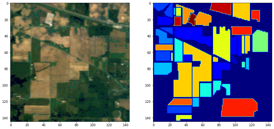
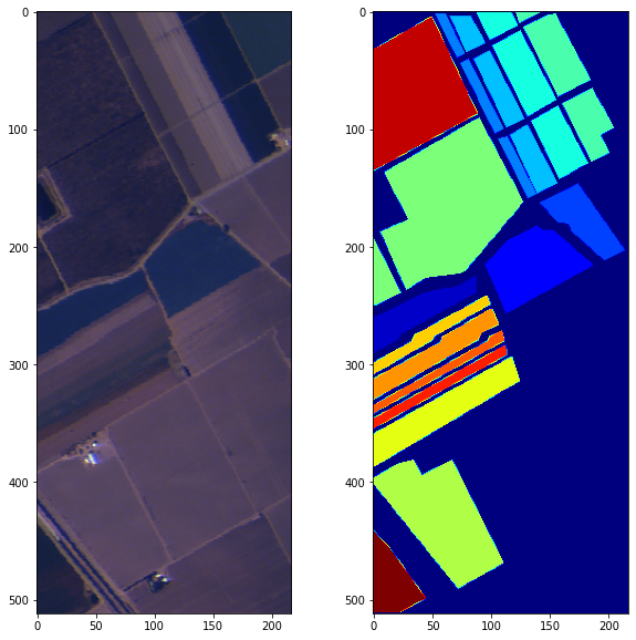
For this project, we had to propose an image processing pipeline to classify pixels in hyperspectral images of crops. Two images and their ground truth were given:
Those images have 200 and 204 spectral bands, respectively. Visualizing hyperspectral images in RGB is not complicated, the only manipulaiton needed is to select images at the corresponding spectral bands (30, 15 and 2 here)
Pipeline
Preprocessing
First of all, the more bands there is, the more the classifying process will be long and complicated; in this sense, the application of a PCA processing which led to dividing by (at least) 2 the number of dimensions by pixel (number bands).
Classification
Then, we have tested a lot of classifying methods: SVMs, Random Forests, KMeans, Spectral Clustering, Hierarchical Clustering, MeanShift, Gaussian methods… But the two bests we came up with were the Nu-Support Vector Classification (NuSVC) and the Random Forest Classifier. During testing phase, we took every pixels into account, but we should have only taken pixels that were not from class 0 (null class, no crop, not classified)
The training set represents 80% of the data, the test set 20%. The training set is used for the training process, the test set is used after training and represents data that was never seen by the classifier before the end of its training.
| ACCURACY | Training Set | Test Set | Mean (reconstuted image) |
|---|---|---|---|
| NuSVC | 0.855 | 0.785 | 0.841 |
| Random Forest | 0.999 | 0.738 | 0.947 |
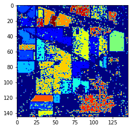
NuSVC result
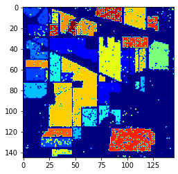
Random Forest result
The table shows that the NuSVC has slightly better results on data it has never seen than the Random Forest, even though the latter performed better on the training set: the Random Forest overfits too much the data it sees.
Postprocessing
When we look at those resulting image, we can see holes in the fields, and spots in the non classified regions: it really looks like noise on an image. So, we applied mathematical morphology. To be more precised, we applied mathematical morphology operations class by class, to avoid fields to fuse together and keep the non-classified delimitations in place.
| ACCURACY | Reconstructed Image |
|---|---|
| NuSVC | 0.866 |
| Random Forest | 0.985 |
NuSVC final results
Random Forest final results
The mean accuracy of both classifier increased with the postprocessing, but the one of the Random Forest really pumped. This final trick was really adapted to its output.


